Neural nets usually construct complex equational surfaces through repeated iterations, each time adjusting the parameters that define the surface. After many iterations, a surface may be "internally" defined that approximates many of the points within the dataset.

The basic function of each neuron is to: (a) evaluate input values, (b) calculate a total for the combined input values, (c) compare the total with a threshold value and (d) determine what its own output will be. While the operation of each neuron is fairly simple, complex behavior can be created by connecting a number of neurons together. Typically, the input neurons are connected to a middle layer (or several intermediate layers) which is then connected to an outer layer, as is seen in Figure 9.

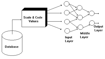
 Figure 11.

To build a neural model, we first train the net on a "training dataset", then use the trained net to make predictions. We may, at times, also use a "monitoring data set" during the training phase to check on the progress of the training.

Each neuron usually has a set of weights that determine how it evaluates the combined strength of the input signals. Inputs coming into a neuron can be either positive (excitatory) or negative (inhibitory). Learning takes place by changing the weights used by the neuron in accordance with classification errors that were made by the net as a whole. The inputs are usually scaled and normalized to produce a smooth behavior.

During the training phase, the net sets the weights that determine the behavior of the intermediate layer. A popular approach is called "backpropagation" in which the weights are adjusted based on how closely the network has made guesses. Incorrect guesses reduce the thresholds for the appropriate connections, as in Figure 12.

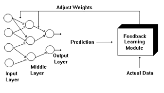
Figure 12.

Neural nets can be trained to reasonably approximate the behavior of functions on small and medium sized data sets since they are universal approximators. However, in practice they work only on subsets and samples of data and at times run into problems when dealing with larger data sets (e.g., failure to converge or being stuck in a local minimum.

It is well known that backpropagation networks are similar to regression. There are several other network training paradigms that go beyond backpropagation, but still have problems in dealing with large data sets. One key problem for applying neural nets to large data sets is the preparation problem. The data in the warehouse has to be mapped into real numbers before the net can use it. This is a difficult task for commercial data with many non-numeric values.

Since input to a neural net has to be numeric (and scaled), interfacing to a large data warehouse may become a problem. For each data field used in a neural net, we need to perform scaling and coding. The numeric (and date) fields are scaled. They are mapped into a scale that makes them uniform (i.e., if ages range between 1 and 100 and number of children between 1 and 5, then we scale these into the same interval, such as -1 to +1). This is not a very difficult task.

However, non-numeric values cannot easily be mapped to numbers in a direct manner since this will introduce "unexpected relationships" into the data, leading to errors later. For instance, if we have 100 cities, and assign 100 numbers to them, cities with values 98 and 99 will seem more related together than those with numbers 21 and 77. The net will think these cities are somehow related, and this may not be so.

To be used in a neural net, values for nonscalar fields such as City, State or Product need to be coded and mapped into "new fields", taking the values 0 or 1 as in Figure 10. This means that the field State which may have the 7 values: {CA, NY, AZ, GA, MI, TX, VA} is no longer used. Instead, we have 7 new fields, called CA, NY, AZ, GA, MI, TX, VA each taking the value 0 or 1, depending on the value in the record. For each record, only one of these fields has the value 1, and the others have the value 0. In practice, there are often 50 states, requiring 50 new inputs.

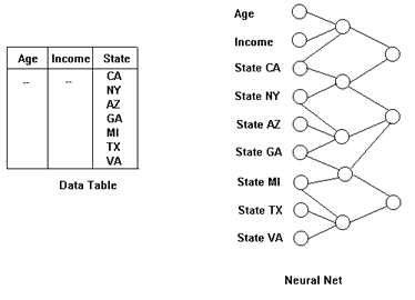
Figure 13.

Now the problem should be obvious: "What if the field City has 1,000 values?" Do we need to introduce 1,000 new input elements for the net? In the strict sense, yes, we have to. But in practice this is not easy, since the internal matrix representations for the net will become astronomically large and totally unmanageable. Hence, by-pass approaches are often used.

Some systems try to overcome this problem by grouping the 1,000 cities into 10 groups of 100 cities each. Yet, this often introduces bias into the system, since in practice it is hard to know what the optimal groups are, and for large warehouses this requires too much human intervention. In fact, the whole purpose of data mining is to find these clusters, not ask the human analyst to construct them.

The distinguishing power of neural nets comes from their ability to deal with smooth surfaces that can be expressed in equations. These suitable application areas are varied and include finger-print identification and facial pattern recognition. However, with suitable analytical effort neural net models can also succeed in many other areas such as financial analysis and adaptive control.

Eventually, the best way to use neural nets on large data sets will be to combine them with rules, allowing them to make predictions within a hybrid architecture.